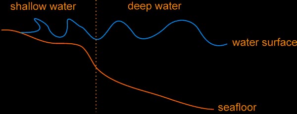
When we try to simulate the behaviour of water surfaces we have to investigate the forces that create these waves. In general we have two different types of forces:
To make things easier we will concentrate in this tutorial on deep water waves and neglect all forces from the interface water-ground (this has to be done anyway, if you would like to create real-time waves). When we describe waves we have to define a few terms:
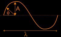
amplitude (symbol:A): determines the height of the
waves
wavelength (symbol: l): determines how
long the wave is
phase (symbol: f): determines the "starting position" of
the wave.
To illustrate this a bit better, I have drawn a couple of waves which differ only in their phase. Beside each wave you find the phase angle in degree (remark: for real calculations you must use radians instead of degrees - > 360° are equivalent to 2*Pi =2*3.1415926535).
The simplest way to simulate a wave is by using a sinus function (like I did in the images above). In 2 dimensions this is quite a nice approximation but how can we generalize it to 3 dimensions? The most primitive way to extend this idea to 3D is by extruding the 2D structure into the 3rd dimension:
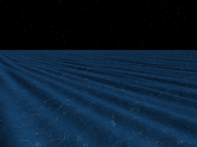
If we look at the image above, it doesn't look like a water surface at all but like a concrete surface. There are two things missing:
If wind blows over a water surface, there are a lot of different waves
with different wavelength and all of them are superimposed and generate
the final image of the water surface. If the wind becomes stronger (i.e.
the wind speed increases), the waves will also change their size
(=wavelength).
Another very important point is that although the main direction of the
waves is determined by the main direction of the wind, there are a lot of
waves whose propagation direction is not exactly parallel to the wind
propagation. This phenomenon limits the width of the waves. The reason for
this phenomenon is that the interaction of wind and water at the water
surface is very complex and in reality it may cause turbulences and other
phenomena which cause small local deviations in the wind direction and
therefore in the propagation direction of the waves.
To simulate a realistic water surface, we have to calculate first the
wavelength distribution (which is the dominant wavelength? which other
wavelength do we have?) and then the angular distribution (how big are the
deviations from the average wind direction?).
To determine these distributions, physicists use a small trick: the
wavelength is related to the frequency f of the wave (the frequency of the
wave tells you how fast the wave mountains and wave valleys change per
second - if you know the propagation velocity of the wave and divide it by
the frequency, you get the wavelength) but it is much easier to calculate
with frequencies. Therefore you calculate all the frequency distributions
and not the wavelength distribution.
For the wavelength distribution there are a couple of models. All of
these models are empirical, which means the scientists observed real water
surfaces, measured the surface elongations and tried to describe the
measurements with a mathematical formalism. This is why all these models
fail under certain circumstances and it is hard to say which model fits
best in the general case. I will show you here the four most prominent
models:
This is - as far as I know - probably the most prominent model. It describes the frequency distribution as a frequency dependent energy function. This is not as complicated as it might look at the first glance. To generate a wave you need some amount of energy (i.e. somebody/something has to do work to generate a wave). If you have a fixed amount of energy and you know that for example 30% of the energy is needed to generate waves with a frequency of 1 Hz (=1 oscillation per second) and the speed of the waves is lets say 4 meters per second, then you know that 30% of the waves have a wavelength of 4 meters (wavelength is velocity divided by frequency). The formula for the energy distribution in this model is:
a = 0.008 and
![]() ,
where g = 9.80665 m/s^2 ( if you drop anything it will fall with the
acceleration g ) and v is the wind velocity. The nice thing about this
model is the formula for fm. fm is the peak frequency of the energy
distribution or in other words: this frequency belongs to the dominant
wave type. In the picture below you see a distribution for a wind speed of
4 m/s.
,
where g = 9.80665 m/s^2 ( if you drop anything it will fall with the
acceleration g ) and v is the wind velocity. The nice thing about this
model is the formula for fm. fm is the peak frequency of the energy
distribution or in other words: this frequency belongs to the dominant
wave type. In the picture below you see a distribution for a wind speed of
4 m/s.
Now that we know the dominant frequency we can calculate the wavelength -
in principle. The problem is that we need the velocity of the wave (you
remember: wavelength is velocity divided by frequency) which we still
don't know. Fortunately there is the dispersion equation for waves
generated by gravitation (put simply: a relation between frequency and
wavelength for water waves):
If we take the calculated energy distribution for a wind velocity of 4 m/s (see plot above), we find a peak frequency of 0.319 Hz. With the dispersion equation we can now calculate the corresponding wavelength and get a numerical value of 15.36 meters.
Like the Pierson-Moskowitz model the Jonswap model offers a special function to calculate the peak frequency:
![]()
The energy distribution is similar but the peak frequency is shifted to a slightly higher frequency and the formula for the energy distribution is more complex:
where g =3.3 and
 .
.
As you can see this model is basically a correction to the Pierson-Moskowitz model, but the drawback is that it needs more computation time to get the results.
where ![]() and b=0.72.
and b=0.72.
This is a third approach to describe deep ocean waves:
where ![]() .
.
In general all 4 models describe the same phenomenon, so you can take which model you want. I prefer the Pierson-Moskowitz model because it is simple, pretty accurate and the energy distribution is nearer to what I would expect from such a phenomenon than the other three models where the first derivative has a discontinuity at the peak frequency (in nature this would be impossible!).
Now that we have the frequency dependent energy distribution, we still need the angular distribution. A nice approach is by using the formula of Mitsuyasu:
Before we start discussing the mathematical details of this
formula lets remember why we need it: this formula describes the
propagation direction of the ocean waves or a bit more precisely it gives
you the energy of a wave with frequency f that is travelling under an
angle q relative to the direction of the wind
(of course you can use this formula also to impress your boy-/girlfriend
;-) The mathematical part needs some more detailed explanations. The first
thing you might be unfamiliar with is the so called gamma function
![]() .
Mathematically this function is defined as
.
Mathematically this function is defined as
Well for many of us the right side of the equation probably doesn't explain much more than the Greek letter on the left side of the equation. I think the simplest way to see what this function does is to calculate a few values:
I suppose you know how it would continue: if you take a
positive integer number n then
![]() .
This function you already know from school as faculty function (of course
you can prove this relation strictly with function theory; the example
above should just help to realize this more intuitively). The important
difference to the faculty function is, that the gamma function is defined
not only for integer arguments as the faculty function but for real valued
arguments. The gamma function is therefore a generalization of the faculty
function. If we go back to the Mitsuyasu formula there is the variable s
which we haven't defined until now. Using the Hasselmann equation we can
define s in the following way:
.
This function you already know from school as faculty function (of course
you can prove this relation strictly with function theory; the example
above should just help to realize this more intuitively). The important
difference to the faculty function is, that the gamma function is defined
not only for integer arguments as the faculty function but for real valued
arguments. The gamma function is therefore a generalization of the faculty
function. If we go back to the Mitsuyasu formula there is the variable s
which we haven't defined until now. Using the Hasselmann equation we can
define s in the following way:
Now that we know the angular distribution from the equations above and the frequency distribution from the Pierson-Moskowitz model discussed earlier we can put everything together and get the total energy distribution:
This is the final result for the Energy distribution as a function of frequency and angle between wind and wave direction. With this result we can finally compute the amplitudes of the waves.
To calculate the amplitudes we use the Fourier transformation. The general idea behind the Fourier transformation is that you can transform equations from the frequency domain to "normal space" and back. You probably get a better idea if we look at a simple example: a satellite is taking images of a landscape with planes, cities etc. and it would be nice if the computer could identify the planes, types of landscape etc. by himself without the help of a human operator. How can this be done? The solution is simple: you make the Fourier transformation of the image (can be done by a simple optical lens) and now you have transformed all the edge information of the structures into bright points at different positions. The position of the points is characteristically for the different structures and all you have to do now is to check whether there are points at a certain position and you can distinguish whether the landscape is a city or agricultural land, whether the plane is a F16 or a MIG21 etc. OK, after taking this small break we can go back to work again ;-) We start calculating the Fourier transformation with the following equation:
dk/df is the first derivative of k and if you remember we have defined k already in the dispersion equation:
If we put everything together we get:
This has to be equal to :
![]()
The last part (
![]() )
is needed to correct a small error we made: the Fourier transformation
should be calculated between plus and minus infinity but we have used it
on a discrete definition area. From this equation we can calculate the a
term which is in fact our holy grail - the formula that gives us (finally)
the amplitude:
)
is needed to correct a small error we made: the Fourier transformation
should be calculated between plus and minus infinity but we have used it
on a discrete definition area. From this equation we can calculate the a
term which is in fact our holy grail - the formula that gives us (finally)
the amplitude:
After all this theory it is probably a good idea to show how you can use all this. Let's start with the implementation of the Gamma-Function.
As mentioned earlier, the Gamma-function is defined as
The most obvious way of calculating the Gamma-function is by numerically integrating the right side of the equation. One possible implementation would be the following:
float gamma(float x)
{
   float integral=0.0f;
   float ulim=10.0f;	// upper integration limit
   float steps=100.0f;	// number of integration steps
   float t;
   for(int i=0; i<ulim; i++)
  {
      t=i/steps*ulim;
      integral+=pow(t,x-1)*exp(-t)*ulim/steps;
   }
   return integral;
}
Nevertheless the numerical integration has some drawbacks: first of all
you have to replace the integral by a discrete sum (which is not very
accurate unless you use very small steps) and the next problem is that you
have to sum up from 0 to infinity (which takes some time ;-) The advantage
is that the exponential function has a negative sign and the entire
function goes to zero. Therefore we don't have to integrate up to infinity
but to a much smaller value (in the example above 10.0) without making a
big mistake. You have to make a trade off between accuracy and speed (high
speed: low value for ulim and steps, high accuracy: high value for ulim
and steps). In this special case I would like to suggest a different
method for the implementation: as I mentioned earlier, the Gamma-function
is a generalization of the faculty function. The Gamma-function of an
integer number is the same as the faculty of the number minus 1, but the
faculty is much easier to calculate and much faster! The only problem is:
what shall we do with non integer numbers? What shall we do with
![]()
for example? 3.9 is almost 4 and therefore it would be a good guess to
calculate it similar to the faculty of 3 (remember:
![]() ):
):
![]()
The correct value would be 5.3, so our approximation is not that bad (and the two multiplications are much faster than the numerical integration of the first method). Can we use this trick in general? What about 3.1? If we handle it in the same way, we get the following result:
![]()
The correct value would be 2.2 - a significant difference and for bigger arguments the discrepancy would become even worth! The problem is, that in this case we shouldn't use 2.1 as the last multiplication factor but something slightly bigger than 1! This is true for all arguments: if the argument is just slightly above the integer number, the last multiplication factor should be somewhere slightly above 1 and if the argument is already near the next higher integer number (like 3.9) the last multiplication factor should be the argument. Putting everything together means that we have to find a linear transformation that maps the interval ]x, x+1] onto the interval [1, x+1] and use the corresponding value from the second interval as the last multiplication factor. With simple linear algebra we get the following transformation equation:
![]()
where ![]() (= the biggest integer number below x). Now we can calculate the faculty
of the argument in a simple loop and we get the last multiplication factor
from the equation above:
(= the biggest integer number below x). Now we can calculate the faculty
of the argument in a simple loop and we get the last multiplication factor
from the equation above:
double gamma (double x)
{
   x=x-1;
   double faculty=1.0f;
   double ulim=x;
   if (floor(x)==x) ulim=x+1.0;
   for(int i=1;i<ulim;i++)
      faculty*=i;
   double fact=floor(x)*x+1.0-floor(x)*floor(x);
   faculty*=fact;
   return faculty;
}
Remember that the Gamma-function of x is not equal to the faculty of x but to the faculty of x-1. Therefore we replace x by x-1.
To get the energy distribution we need the Mitsuyasu distribution and the Pierson-Moskowitz formula. Let's start with the Mitsuyasu distribution:
double MitsuyasuDistribution (double f, double theta)
{
   double s,D;
   double ang=cos(theta/2);
   ang *=ang;                   // calculate square of cos(theta/2)
   if (f<fPeak)                 // frequency peak fpeak is globally defined
   {
      s=9.77*pow(f/fPeak,-2.5);
   } else
   {
      s=6.97*pow(f/fPeak,5.0);
   }
   D=Gamma(s+1)*pow(ang,s)/(2*sqrt(Pi)*Gamma(s+0.5));
   return(D);
}
In this function I used the global variable fPeak which represents the peak frequency of the wavefrequency distribution. We will calculate it's value in the InitWater function. Please keep also in mind that all the implementations I show here are not optimised for speed. I rather tried to keep it easy understandable (in a game you would probably replace the 2*sqrt(Pi) part with the actual number, the division by 2 with a shift operation etc.). The next function we need is based on the Pierson-Moskowitz formula:
double EPM(double f)
{
   double EPM;    // EPM=Energy according to the Pierson-Moskowitz formula
   EPM=alpha*g*g*exp(-1.25*pow(f/fPeak,-4))/pow(2*Pi,4);
   return EPM;
}
The implementation of this function is straight forward, so I don't have to explain much. The only thing I would like to explain are the constants. Alpha is a constant needed in the Pierson Moskowitz formula and it's value is 0.0081. g is the gravitational acceleration and the theoretical standard value is 9.80665. This is an average value at sea level (g is actually a function of height - the higher you are, the smaller is g usually). If you want to make precise simulations (i.e. simulate the behaviour of a ship in a storm), you might want to take care of this problem (however the real values of g are always around 9.8 as long as you are on sea level). The product of the two functions above gives us now the energy distribution:
double EnergyDistribution(double f, double theta)
{
   return EPM(f)*MitsuyasuDistribution(f,theta);
}
The next step is to calculate the amplitude of the wave from the energy distribution:
double Amplitude(double f, double theta, double k)
{
   double omega = 10.0;            // area of the water surface part
   double amp;                     // amplitude of the wave
   amp=sqrt(EnergyDistribution(f,theta)*g*Pi*Pi/(k*f*omega));
   return amp;
}
omega is the area of the water surface part and k is the wave vector (defined as 2*Pi/wavelength of the wave) which we will determine in the InitWater function.
Before we can start initialising the wave parameters, we have to define a structure WAVE:
typedef struct
{
   double direction;
   double dirX;
   double dirY;
   double lambda;                 // wavelength
   double k;                      // wave number: k=lambda/(2*Pi)
   double omega;                  // angular frequency: omega=2*Pi*f
   double freq;                   // frequency
   double periode;                // periode of the wave
   double amplitude;              // amplitude of the wave
   double phase;                  // phase of the wave
} WAVE;
As you can see there is a lot of redundant information in this structure (i.e. freq, omega and periode is essentially the some and the only difference between lambda and k is a factor of 2*Pi). The reason why we do this is, that we don't have a lot of different waves (so we don't waste much memory) but we need the different variables very often ( so we can increase the speed by just calculating once the different combinations (i.e. freq, omega,…) and then just using the proper variable). Now we can start initialising the parameters and calculating the waves:
void InitWater()
{
   fPeak=0.13*g/WindSpeed;         // calculate peak frequency
   WAVE *w = &wave[0];
   nWaves=0;                       // number of useable waves calculated so far

   while (nWaves<maxwave)
   {
      float f = fPeak + rand() / 16384.0f * 0.5 - 0.5;

      if (f>0.0)
      {
          w->lambda      = 2.0*Pi/(pow( 2.0*Pi*f,2.0)/g);
          w->k           = 2.0*Pi/w->lambda;
          w->omega       = sqrt(g*w->k);
          w->freq        = w->omega / (2.0*Pi);
          w->periode     = 1.0f/w->freq;
          w->direction   = (rand()/16384.0f+0.5f)*Pi;
          w->dirX        = cos(w->direction)*0.5f;
          w->dirY        = sin(w->direction)*0.5f;

          double phi0    = rand()/16384.0f*Pi;
          double a0      = Amplitude(w->freq,w->direction-WindDirection,w->k);

          w->amplitude   = a0*cos( phi0 );
          w->phase       = a0*sin( phi0 );

          if (fabs(w->amplitude)>=0.0001f )
          {
             w ++;
             nWaves ++;
          }
      }
   }

   for (int i=0; i<WaterX*WaterY; i++ )
   {
      WaterNormal[ i ].x = 0.0f;
      WaterNormal[ i ].y = 1.0f;
      WaterNormal[ i ].z = 0.0f;
   }
}
First we calculate the peak frequency and in the while loop we calculate the parameters of potential wave candidates which we generate randomly. All the negative frequency we drop immediately because they have no physical meaning. If the frequency is positive (i.e. the wave really exists), we check whether the amplitude of the wave is big enough, so that this wave will give a significant contribution (fabs(w->amplitude)>=0.0001). If the wave is big enough we increase the pointer (w++) and the number of waves (nWaves++) and calculate the next wave. When we have found all the waves, we initialize the surface normals for all the water elements (needed for the graphics output later on)
Here you will find a new tutorial on how to implement the algorithms above graphically. In the meantime you can download a demo, that he has made fora german Computer magazin (PC-Magazin).