One of the most demanding tasks when you try to simulate a natural
environment (for example for games or rendering aplications) is the
simulation of plants. How can you create a realistic plant that interacts
with its environment as a real plant would interact? There have been a
couple of different approaches but only one of them has been really
sucessfull in simulating a broad variety of different plants - the so
called L-systems.
The L-systems - or Lindenmayer systems - have been developed by the
biologist Aristid Lindenmayer. His idea was to simulate plants by a model
that corresponds as accurately as reasonably possible to the real growth
of plants. If we take a look at the growth of real plants, they start with
some sort of seed (in the L-system terminology this is called an axiom).
The cells of this seed reproduce themselves according to some rules which
are determined by the DNA (=desoxyribonucleic acid) and finally create the
entire plant. Of course this is a pretty oversimplified view of what is
really happening, but for creating an usefull model this is already enough
accurate.
Let's start with one of the most prominent examples, that is used in all
books about this topic to show the power of L-systems:

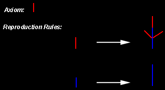
The beauty of this L-system is, that it is extremely
simple. There are only two different elements (in this example represented
by the blue and the red line) : the red line represents the younger parts
of the plant, while the blue line represents the older part of the plant.
It is therefore quite reasonable to start with the younger part (i.e. use
the red line as axiom). The first reproduction rule (the one for the red
line) states, that with each iteration the young part grows by a factor of
two and becomes an old part (the red line is replaced by two blue lines).
Additionally three new young branches (the three red lines) grow from this
old part. The second reproduction rule tells, what happens to old parts:
they simply grow, but no new branches are formed (one blue line is
replaced by two blue lines). This behaviour is also what you would expect
from a real plant: it is highly unlikely that after some time a new leave
emerges from the stem of an old tree - the probability that the leaves
starts at some new branch is much higher.
OK, after we now basically understand how this L-system works, lets take
a look at the result:

In the image above I have drawn the red and blue lines as green, so that
it reminds a bit more to a plant. The starting point (n=0) is just the
axiom (i.e. a straight line corresponding to the red line of the axiom
which represents the new part of the grass). In the first iteration (n=1)
the replacement rule for the red line is applied (there is no blue line,
that could be replaced because the axiom was only one single red line) and
we get an old stem from which 3 young branches emerge. In the second
iteration (n=2) the two blue lines of the stem are replaced by 4 blue
lines (i.e. the old stem grew) and each branch is replaced by a stem from
which 3 new branches emerge. If you do this for another 6 iterations you
end up with something that looks pretty similar to some sort of grass.
As you can see we can already get very nice results with quite simple
models. The only three things we have asumed about this grass were, that
However if you really want to generate these plants on your computer,
you have to use a little bit more formal aproach (although the colorful
lines look nice, the computer is usually not to happy with them ;-)
Lindenmayer suggested to represent each different element of the plant by
a different letter (for example the red line would be represented by F and
the blue one by G). To represent the actual branching structure you need
additionally some geometrical representation. Lindenmayer sugested to use
turtle graphics for this representation. Originally turtle graphics has
been used in an old programming language (called LOGO), that probably most
of us haven't seen any more. Nevertheless the idea behind is very
intuitive and most people will recognize it immediately because many games
use it to control the movements of the actors or some rendering programs
use it also for their realtime preview.
The idea is, that you sit on the turtle and tell her to go straight ahead
(default mode, each capital letter means that a straight line of unit
length has to be drawn), turn left (in the L-system represented by +) or
turn right (in the L-system represented by -). When you turn left or
right, you just change the orientation of the turtle but you don't draw a
line in that direction. For example to draw a line to the left, you have
to use the sequence +F instead of just +. If you want to have branches,
you need an additional symbol (in L-systems represented by [ ) to put the
current position of the turtle into the stack and a symbol (in L-systems
represented by ] ) to get the position of the turtle back from the stack
after the branch has been drawn.
With these conventions the L-system above would look like this:
derivation length: 8
Axiom: F
F --> G[+F][-F]GF
G --> GG
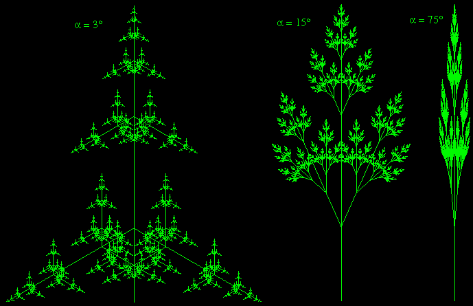
Beside the actual L-system there are a few additional informations needed on how the L-system has to be interpreted. In the L-system above we have to specify the angle by which the orientation is changed with + or -. As you can see this affects the final result quite significantly:

The symbols mentioned above are already a good starting point, but if you want to create more complex models (3D models, flowers,...) you need a little bit more symbols. In the following list you can find the most important symbols for L-systems with a short description of each (see also the paper "Visual models of plant growth" from Prusinkiewicz et al.):
| F(s), G(s) | Move forward a step of length s and draw a line segment from the original to the new position of the turtle. |
| f(s), g(s) | Move forward a step of length s without drawing a line. |
| @O(r) | Draw a sphere of radius r at the current position. |
| +(a) | Turn left by angle a around the z axis. The rotation matrix is Rz(a). |
| -(a) | Turn right by angle -a around the z axis. The rotation matrix is Rz(-a). |
| &(a) | Pitch down by angle a around the y axis. The rotation matrix is Ry(a). |
| /\(a) | Pitch up by angle -a around the y axis. The rotation matrix is Ry(-a). |
| /(a) | Roll left by angle a around the x axis. The rotation matrix is Rx(a). |
| \(a) | Roll right by angle -a around the x axis. The rotation matrix is Rx(-a). |
| | | Turns 180° around the z axis. This is equivalent to +(180) or -(180). |
| [ | Push the current state of the turtle (position, orientation and drawing attributes) onto a pushdown stack. |
| ] | Pop a state from the stack and make it the current state of the turtle. No line is drawn, although in general the position and orientation of the turtle are changed. |
| { | Start saving the subsequent positions of the turtle as the vertices of a polygon to be filled. |
| } | Fill the saved polygon. |
| ~X(s) | Draw the surface identified by symbol X, scaled by s, at the turtle's current location and orientation. Such a surface is usually defined as a bicubic patch. |
| #(w) | Set line width to w, or increase the value of the current line width by the default width increment if no parameter is given. |
| !(w) | Set line width to w, or decrease the value of the current line width by the default width decrement if no parameter is given. |
| ;(n) | Set the index of the color map to n, or increase the value of the current index by the default color increment if no parameter is given. |
| ,(n) | Set the index of the color map to n, or decrease the value of the current index by the default color decrement if no parameter is given. |
The rotation matrices mentioned in the above definitions are defined as follows:

The definitions above represent the symbol definitions according to Lindenmayer (and extended by Prusinkiewicz). It is a good idea to use these definitions for your own implementations too, because it is much easier this way to exchange the L-systems with fellow programmers/scientists.
Well now you know everything you need to let the plants grow on your
desktop. When you want to actualy grow plants now, you have to either
implement the string replacement and graphic output routines or you can
use one of the available programs. The best programm you can use is
LinSys3D
developed by Andrea Esuli.
All three programs are very similar and pretty powerfull. I will now
briefly describe how you can create L-systems in one of these programs.
Typically the L-system would look like this:
derivation length: 8     //the number of derivation steps
Axiom: F                 //the axiom
F --> G[+F][-F]GF        //one (or more) productions
G --> GG
Additionally to the actual L-system you need some parameters for the graphical interpretation. For the L-system above, these are:
angle increment: 15              //the turning angle, in degrees
initial line width: 1 pixels     //… self-explanatory
initial color: 2                 //index to the color map (2=green)
scale factor: 0.9000             //controls the size on the screen
The commands above will produce the simple gras we discussed earlier. By modifying the code above you can easily represent any L-system you want.
As we have seen L-systems are a very powerfull tool to model plants.
Nevertheless I have to admit that finding a proper model for a certain
plant is usually quite time consuming (at least for non-biologists like me
;-) When you want to model a new plant you should have a couple of photos
(or even better: the plants itself) in different growth phases. Then you
have to compare from which part which other parts are developed and then
you can asign to each element a letter and you must try to find the rules
that govern the development. Additionally you should try to keep the axiom
as simple as possible (don't put all your knowledge into the axiom - the
axiom should not be the final plant but the seed for the plant! ).
Let's try to create some sort of fern as an example:

If you look at the final plant it is usually much to
complex to get a good idea on how to design the L-system. Therefore you
should try to get a few images of the plant as it looks in an early state.
There is also another principle, that might help you sometimes:
selfsimilarity. Put simply, this means that if you take a small part of
the plant, the structure will be similar to the structure of the entire
plant (this principle has been discussed very extensively in the context
of fractals).
In most plants you don't find this phenomenon, but in some plants - like
ferns - this principle is obvious and helps you designing the L-system:
you don't necesarily need images of all the different states of the plant,
but it is suficcient to concentrate on a small part of the plant. Let's
take a look at a small part of a single leaf :

Based on what we know so far, the most obvious approach would be something like this:
Axiom: F
F --> FF[+FFFF][-FFFF]FF[+FFF][-FFF]FF[+FF][-FF]FF[+F][-F]FFFF
Sure this type of L-system would reproduce the leaf above, but as you
might guess it is not very desireable to put all your knowledge in one
universal super reproduction rule. The development should be governed by
some simple principles. If we take a closer look at the leaf above, we
see, that the lower branches could be described as older parts, that had
more time to grow, while the upper branches are the newer ones. Of course
this could also be implemented with the ideas we have discussed so far
(just use a couple of different letters for the different growth phases).
However I would like the chance to show you a new concept, that is very
useful in such cases: parametric L-systems. The idea is, that you
determine the age of the element by an additional numerical parameter.
With this notation the L-system might look like the following:
Lsystem: 0
derivation length: 30
Axiom: A(0)
A(d) : d>0 --> A(d-1)
A(d) : d==0 --> F(1)[+A(4)][-A(4)]F(1)A(0)
F(a) --> F(1.25*a)
endlsystem
On the first glance this might look a bit confusing, but on the second
glance you'll see, that it is much simpler and more elegant than the brute
force approach above. As we would do in the classical case, we introduce
two different letters for the two different parts we have in the plant -
the old parts, which are just growing straight but are not capable of
making any new branching strucutres (represented by F) and the young
parts, that are responsible for the branching (represented by F).
The parameter behind F represents the length of the straight element. By
multiplying it each time with the factor 1.25 we simulate the growth of
this element. The higher this parameter, the faster this element grows and
vice versa. The actual value has to be adjusted later during the
simulation. Until you know (from the simulation) what value makes sense,
you should start with an average growth rate of 25% (i.e. a multiplication
factor of 1.25). If this value is too small, all the leaves will overlap,
while a too big value creates large empty spaces (it will remind you to a
tree in winter ;-)
For the branching element we need two rules the first one is responsible
for the aging (A(d) : d>0 --> A(d-1)), while the second one takes
care of the actual branching: if the A-parameter is equal to 0 (i.e.: the
element is old) it is replaced by the actual branching structure. As you
can see we have used 4 as new A-parameter for the branches in the second
reproduction rule. Keep in mind that A is responsible for the branching
and that the A-parameter is therefore proportional to the density of the
branches. If you don't have a feeling which parameter might be usefull,
you should start with a big value like 10 and decrease this value until
the density of the branches is like you want it to be (if you start with a
small value, the calculation of the L-system might take eternities :-) In
this case I know from Lindenmeyers book "Algorithmic beauty of plants",
that 4 is a reasonable parameter in this case ;-)
If we simulate this L-system we get the following image:

As you can see this image looks already pretty similar to a fern. Nevertheless the spacing between the leaves is a little to big. If we therefore reduce the growth factor from 1.25 to say 1.23 we get a more realistic picture:

The corresponding L-system would be:
derivation length: 30
Axiom: A(0)
A(d) : d>0 --> A(d-1)
A(d) : d==0 --> F(1)[+A(4)][-A(4)]F(1)A(0)
F(a) --> F(1.23*a)
and as viewing parameters I used the following (in L-Studio again):
angle factor: 15
initial color: 3
initial line width: 1
I hope that this tutorial gives you a starting point for
your own experiments with L-systems and helps you creating your own plant
simulations. In another tutorial we will discuss the more advanced aspects
of L-systems (i.e.: how can we create asymmetrical plants? How can we
avoid, that all the plants of one type look identical? How can we simulate
environmental influences on the plant? ...).
If you need some inspiration, you should check out the demo of
Vue
d'Esprit: they have a very good rendering tool, which is capable of
rendering highly realistic plants!
When you have created a good plant and you would like to share your work with others, send me your L-system (including the viewing parameters) and I will add it here.